How to Create a Choropleth Map in Python (without GeoPandas, GiS, or any GeoJSON knowledge)
I don’t know if it’s because GeoPandas is poorly maintained or that most people can’t be bothered and simply use GiS software for this type of problem, but I couldn’t for the life of me create some simple informative maps in Python. After quite a bit of searching and many hours of trial and error, here’s a quick and easy way to create a Choropleth map with pretty much only Python knowledge.
Quickly, here are the imports I’m running and the versions of each:

To create a useful Choropleth map, you’re likely going to need two datasets: a map (GeoJson, Shapefile, KML, etc.) and data you want to put on the map (Pandas DataFrame, series, etc.). Your map will, at some point, need to be converted into a GeoJSON file (which will later be turned into a JSON). Don’t worry if you don’t know anything about JSONs; they look and act like dictionaries.
Most often, when you’re looking for map data online, a website will offer a download in the form of GiS-readable maps, but no CSVs or anything that’s readily readable into Python. This shouldn’t be an issue. There are many websites that can convert Shapefiles, KMLs, and more into GeoJSONs, which is how this example will move forward (be careful to check that you trust downloading from any of the sites that you use).
An important note: When converting files, you will normally have the option to select which projection coordinate system (normally as an EPSG code) your file is currently written in and which you would like it to be downloaded in. If you don’t feel like learning this, just know that EPSG 3857 is one of the more popular projection coordinate systems (used by Google Maps and Open Street Maps), followed closely by 4326 and 7789.
Now, once you’ve actually got the data you want to work with, you’ve got to perform basic EDA with one important fact in mind: whatever map-based factor you’re mapping your data on (ZIP codes, county lines, national borders) needs to match in both datasets. I’ll show you what I mean.
In this example, we want to show the number of jobs in Chicago, grouped by ZIP code. The data for this was pulled from the City of Chicago’s data portal as well as the annual Illinois Department of Employment Services “Where Workers Work” report. We’re mapping based on ZIP codes, so whatever ZIP codes I have in my job data need to match a ZIP code in my map data or else it will have nowhere to go.
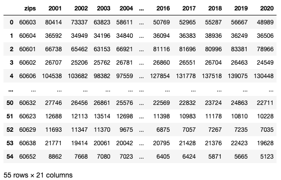
After imputing values for 2001 ZIP codes 60661 and 60606 using a linear regression and doing various other cleaning, we ended up with this DataFrame:

What was important was that the names of my 55 columns matched with a key in my json file. Here’s how it was read in:
import jsonwith open('./datasets/zip_codes.geojson') as f:
    zips_map = json.load(f)
The zips_map variable is a dict type and can be interpreted as such by a Python programmer. The first few lines of zips_map appear as follows:
{'type': 'FeatureCollection',
 'features': [{'type': 'Feature',
   'properties': {'objectid': '33',
    'shape_area': '106052287.488',
    'shape_len': '42720.0444058',
    'zip': '60647'},
   'geometry': {'type': 'MultiPolygon',
    'coordinates': [[[[-87.67762151065281, 41.917757801062976],
       [-87.67760690174252, 41.91734720847048],
       [-87.67760511932958, 41.91730238504324],
       [-87.67760063005984, 41.917188199438144],
       [-87.67759765058332, 41.916991119379674],
       [-87.67759310412458, 41.91669230188045],
       [-87.6775879922483, 41.91640204306182],
       [-87.67758757917139, 41.91637778172058],
       [-87.677586292912, 41.91623784614856],
       [-87.67758575813848, 41.9161788147321],
       [-87.67758053649547, 41.91594236952244],
       [-87.677578323991, 41.91584265904772],# ...and so on
The important thing we’re looking for here is the ZIP code. In order to compare both datasets’ ZIP codes, we’ll make a list of either and convert them into sets to compare the uncommon values:
job_data_zips = list(jobs.columns)
geojson_zips = sorted([int(zips_map['features'][i]['properties']['zip']) for i in range(len(zips_map['features']))])set(geojson_zips) ^ set(job_data_zips)# Output:
{60610, '60610 & 54', 60627, 60635, 60642, 60654, 60707, 60827}
The first thing that jumps out here is the string '60610 & 54'. We can see that both 60610 and 60654 are present in the output as well. So it’s clear that one dataset combined these two ZIP codes into one column, while another kept them separate. At this point, we’ve got to work through each of the items in the output to see why exactly they only appear in one of the two datasets. Domain knowledge would help significantly at this step, which ended up being the most time consuming part. Fun fact: the town of Elmwood Park, a Chicago suburb, changed its ZIP code from 60635 to 60707 more than 25 years ago out of a sense of community identity (Chicago Tribune article).
Once you work through all of these discrepancies and the output of our last code cell above is an empty set, we can actually move on to the mapping. I saved my datasets to my workspace as follows:
jobs.to_csv('./datasets/jobs_data_cleaned.csv')with open('./datasets/zips_map_cleaned.json', 'w') as fp:
    json.dump(zips_map, fp)
The mapping itself is relatively straightforward. This is where your specific use case is going to dictate most of the parameters and choices you make. I’ll show what I did and also give a few troubleshooting tips.
import pandas as pd
import folium
import jsonjobs = pd.read_csv('./datasets/jobs_data_cleaned.csv', index_col=0)# rearranging DataFrame to work with mapping code that's coming up
jobs = jobs.T.reset_index(level=0)
jobs.columns = ['zips'] + ([i for i in range(2001,2021)])# layout of DataFrame for reference
pd.set_option('display.max_row', 10)
pd.set_option('display.max_column', 10)
jobs
divisions=[0,0.25,0.5,0.75,0.98,1]quantiles = list(jobs[2001].quantile(divisions))m = folium.Map(location=[41.881832, -87.623177], tiles='openstreetmap', zoom_start=10)folium.Choropleth(
    geo_data=zips_map,
    name='2001',
    data=jobs,
    columns=['zips', 2001],
    key_on='properties.zip',
    fill_color='YlGn',
    fill_opacity=0.7,
    line_opacity=0.3,
    bins=quantiles,
    legend_name=f'Number of Jobs by ZIP Code in 2001',
).add_to(m)m
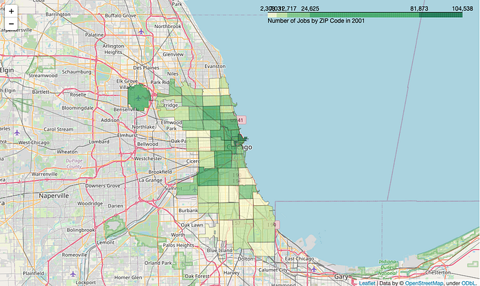
Let’s explain a little bit about what’s going on in that code. First of all, the divisions and quantiles variables are customizable to how you want your data split up. This is small but also the most crucial part of your dataviz. folium.Choropleth defaults to 6 bins of equal size. This can cause the exact same data to look completely different, so it’s important to keep ethics in mind while choosing your bin size in regards to what effects you’re creating with the implications from your dataviz.
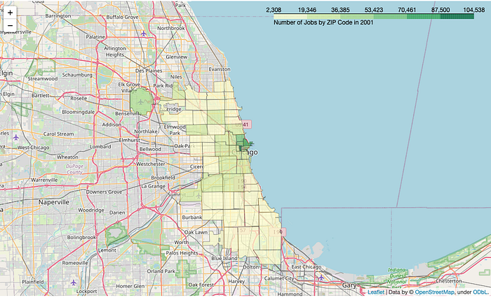
Another important note is that your fill_color parameter is incredibly important to the functionality of your code. Here, I chose 'YlGn' to clearly stand out against the street map on this scale, but note that this color (or any other multihue argument from colorbrewer) can only map between 3 and 9 levels (I have 5 in my first graphic then 6 in my second). This can be further customized if you know a bit about style functions and colorbrewer, but just be mindful of whether your data is quantitative or qualitative and how many levels you have when choosing your fill_color. Be mindful of colorblind folks as well (red-green color blindness being the most common, followed by blue-yellow).
This base level of Choropleth understanding can be expanded upon to create much more advanced and interactive graphics, including some with removable layers and multiple data frames, or simply turned into a .gif as I did above. The options are truly endless.