A Quick and Customizable Function to GridSearch Over ARIMA Model Parameters in Python

One of the things that I came to discover during the process of modelling time series is that the most time consuming part is choosing how exactly to model a function. With ARIMA models, your forecast is created from the sum of two models, an Autoregressive and Moving Average model, and (possibly) an integrated section for data that needs to be differenced to induce stationarity. The function is as follows:

Fine tuning these parameters, namely the order of the ARIMA model (p,d,q) can be a lengthy challenge of trial and error. Through my time spent studying this method of time series modelling, I decided to automate the process. I’ll include the code below, but here’s the GitHub repo for a more readable version: https://github.com/mdsexton/ARIMA_function
Note that this code was designed to run in an iPython Notebook.
This function is designed to automate the process of choosing an ARIMA model with the lowest AIC score. It’s designed to be used on stock tickers from the yfinance module, but could easily be edited for other applications. It's mostly customizable. All there is to do is to insert your data, choose your start and end dates, and enter the list of p, d, and q values you'd like to "GridSearch" over. It will test all combinations of these three scores while continually updating the best model. Outside knowledge of the pitfalls of ARIMA models is reccommended since not all factors (such as seasonality) are accounted for here.
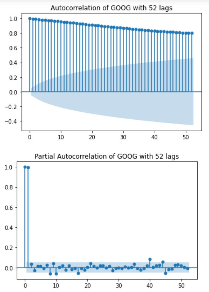
Once all models are tested, the resulting AIC score, along with MSE, RMSE, and R² score of both the training and testing data are displayed. Additionally, the results of the Augmented Dickey-Fuller test show whether the data is stationary or not. Autocorrelation is checked with ACF and PACF graphs. Lastly, the model forecasts and residuals are plotted out.
The example in the iPython notebook uses GOOG stock prices from 2015 through 2020. I chose to iterate over p and q values from 0 to 5 and d values from 0 to 2.
This code produces several warnings due to issues with the use of datetime information in the index of the data, so I’ve included a chunk of javascript code that allows you to toggle them.
source for the javascript code below: https://stackoverflow.com/questions/9031783/hide-all-warnings-in-ipython
%%javascript
(function(on) {
const e=$( "<a>Setup failed</a>" );
const ns="js_jupyter_suppress_warnings";
var cssrules=$("#"+ns);
if(!cssrules.length) cssrules = $("<style id='"+ns+"' type='text/css'>div.output_stderr { } </style>").appendTo("head");
e.click(function() {
    var s='Showing';
    cssrules.empty()
    if(on) {
        s='Hiding';
        cssrules.append("div.output_stderr, div[data-mime-type*='.stderr'] { display:none; }");
    }
    e.text(s+' warnings (click to toggle)');
    on=!on;
}).click();
$(element).append(e);
})(true);
.
import numpy as np
import pandas as pd
import matplotlib.pyplot as pltimport yfinance as yf
from sklearn.metrics import mean_squared_error as mse, r2_score
from IPython.display import display, Markdownfrom statsmodels.tsa.arima.model import ARIMA
from statsmodels.graphics.tsaplots import plot_acf, plot_pacf
from statsmodels.tsa.stattools import adfuller
.
def best_ARIMA(ticker, start_date, end_date, p_values, d_values, q_values, feature='Adj Close', test_size=0.9, lag_number=52, adf_alpha=0.01):
# reading in closing stock info
stock = yf.download(ticker, start=start_date, end=end_date)df = pd.DataFrame(index=pd.date_range(start=start_date, end=end_date))
df = stock[feature]
df.dropna(inplace=True)
# train test split
split_index = round(len(df) * test_size)
train_end_date = df.iloc[[split_index - 1]].index[0].strftime('%m-%d-%Y')
test_start_date = df.iloc[[split_index ]].index[0].strftime('%m-%d-%Y')
train = df[:split_index]
test = df[split_index:]
# Starting values for AIC and ARIMA order
best_aic = 1e20 # arbitrarily large value
best_p = 0
best_q = 0
best_d = 0
print(f'Testing {len(p_values) * len(d_values) * len(q_values)} different ARIMA models...')
for p in p_values:
for d in d_values:
for q in q_values:
#print(f'Checking AIC improvement in ARIMA({p},{d},{q})')
# ^ uncomment if you want to see each iteration as it happens
try:
model = ARIMA(train, order=(p,d,q)).fit()if model.aic < best_aic:
best_aic = model.aic
best_p = p
best_d = d
best_q = q
'''
This section can be uncommented if you want to see
which ARIMA models improve the AIC score and
by how much.
print(f'ARIMA({p},{d},{q})')
print(f'AIC: {best_aic}')
print(f'Training RMSE: {rmse(train[d:], train_preds, squared=False):.3e}')
print(f'Testing RMSE: {rmse(test, test_preds, squared=False):.3e}')
print()
'''except np.linalg.LinAlgError:
print(f'LinAlgError: SVD in ARIMA({p},{d},{q}) does not converge.')except ValueError:
print(f'ValueError: The computed initial AR coefficients are not stationary for ARIMA({p},{d},{q})')# after all p, d, and q value combinations are iterated over
print('##################################################')
print('Modelling completed')
train_preds = model.predict(train.index[d], train.index[-1])
test_preds = model.forecast(steps=len(test))
residuals = test.values - test_preds.values
display(Markdown(f'Lowest AIC Model:'))
display(Markdown(f'ARIMA({best_p},{best_d},{best_q})'))
display(Markdown(f'AIC: {best_aic}'))
print()
display(Markdown(f'Training MSE: {mse(train[d:], train_preds):.3e}'))
display(Markdown(f'Testing MSE: {mse(test, test_preds):.3e}'))
print()
display(Markdown(f'Training RMSE: {mse(train[d:], train_preds, squared=False):.3e}'))
display(Markdown(f'Testing RMSE: {mse(test, test_preds, squared=False):.3e}'))
print()
display(Markdown(f'Training $R^2$: {r2_score(train[d:], train_preds):.3e}'))
display(Markdown(f'Testing $R^2$: {r2_score(test, test_preds):.3e}'))
print()# show ACF and PACF plots
if lag_number >= len(df):
print(f'Error: lag number too large. Max lag amount of {len(df) - 1} used instead')
plot_acf(df, lags=len(df) - 1)
plt.title(f'Autocorrelation of {ticker} with {lag_number} lags')
plot_pacf(df, lags=len(df) - 1)
plt.title(f'Partial Autocorrelation of {ticker} with {lag_number} lags')
print()
else:
plot_acf(df, lags=lag_number)
plt.title(f'Autocorrelation of {ticker} with {lag_number} lags')
plot_pacf(df, lags=lag_number)
plt.title(f'Partial Autocorrelation of {ticker} with {lag_number} lags')
print()
# show results of the Augmented Dickey-Fuller test for stationarity
test_results = pd.Series(adfuller(df.dropna())[0:2], index=['Test Statistic','p-value'])
if test_results[1] <= adf_alpha:
display(Markdown('Augmented Dickey-Fuller test results:'))
print(test_results)
display(Markdown(f'With an $\\alpha$ level of {adf_alpha} amd a $p$-value of {test_results}, we reject the null hypothesis and assume that the data is stationary.'))
else:
print('Augmented Dickey-Fuller test results:')
print(test_results)
display(Markdown(f'With an $\\alpha$ level of {adf_alpha} amd a $p$-value of {test_results}, we fail to reject the null hypothesis and assume that the data is not stationary.'))
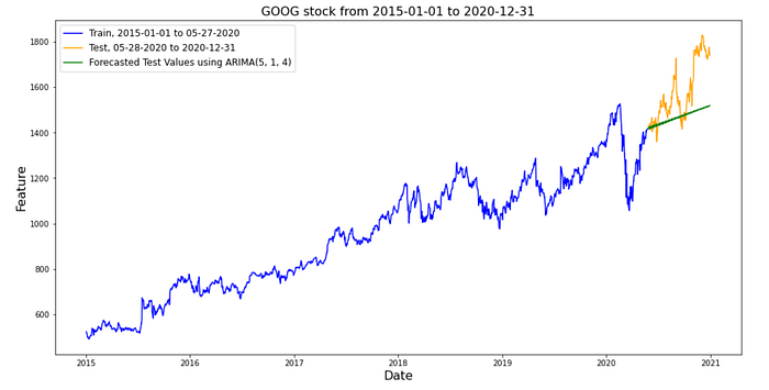
# showing a graph of our forecast vs the actual values
plt.figure(figsize=(16,8))
plt.plot(train.index, train, color='blue', label=f'Train, {start_date} to {train_end_date}')
plt.plot(test.index, test, color='orange', label=f'Test, {test_start_date} to {end_date}')
plt.plot(test.index, test_preds, color='green', label=f'Forecasted Test Values using ARIMA({best_p}, {best_d}, {best_q})')plt.title(f'{ticker} stock from {start_date} to {end_date}', size=16)
plt.xlabel('Date', size=16)
plt.ylabel('Feature', size=16)
plt.legend(fontsize=12)
plt.show();
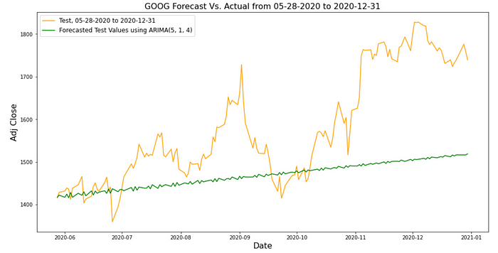
# zooming in on just the test forecast and actual values
plt.figure(figsize=(16,8))
plt.plot(test.index, test, color='orange', label=f'Test, {test_start_date} to {end_date}')
plt.plot(test.index, test_preds, color='green', label=f'Forecasted Test Values using ARIMA({best_p}, {best_d}, {best_q})')
plt.title(f'{ticker} Forecast Vs. Actual from {test_start_date} to {end_date}', size=16)
plt.xlabel('Date', size=16)
plt.ylabel(f'{feature}', size=16)
plt.legend(fontsize=12)
plt.show();
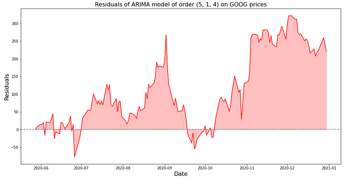
#plot residuals of test values
plt.figure(figsize=(16,8))
plt.title(f'Residuals of ARIMA model of order ({best_p}, {best_d}, {best_q}) on {ticker} prices', size=16)
plt.xlabel('Date', size=16)
plt.ylabel('Residuals', size=16)
plt.plot(test.index, residuals, color='r')
plt.axhline(y=0, color='grey', linestyle='dashed')
plt.fill_between(test.index, residuals, 0, color='r', alpha=0.25)
plt.show();
return
.
%%time
p = range(6)
d = range(3)
q = range(6)best_ARIMA('GOOG', '2015-01-01', '2020-12-31', p, d, q)
To finally produce this output:
[*********************100%***********************]  1 of 1 completed
Testing 108 different ARIMA models...##################################################
Modelling completedLowest AIC Model:ARIMA(5,1,4)AIC: 11455.995335706286Training MSE: 2.703e+02Testing MSE: 2.307e+04Training RMSE: 1.644e+01Testing RMSE: 1.519e+02Training 𝑅2R2: 9.957e-01Testing 𝑅2R2: -4.056e-01Augmented Dickey-Fuller test results:
Test Statistic   -0.404273
p-value           0.909383
dtype: float64With an α level of 0.01 and a p-value of 0.909383, we fail to reject the null hypothesis and assume that the data is not stationary.
I hope that you find this useful and that it’s able to speed up your modelling process.